SUMMARY. critical region Z* Z-critical value Decision errors Type I: you reject the null, but you shouldn't. (α) Type II: You do not reject the null,

Prezentace na téma: "SUMMARY. critical region Z* Z-critical value Decision errors Type I: you reject the null, but you shouldn't. (α) Type II: You do not reject the null,"— Transkript prezentace:

1 SUMMARY

2 critical region Z* Z-critical value

3 Decision errors Type I: you reject the null, but you shouldn't. (α) Type II: You do not reject the null, but you should. Decision Reject H 0 Retain H 0 State of the world H 0 true Type I error FP H 0 false Type II error FN

4 Summary of t-tests two-sample tests

5 NEW STUFF

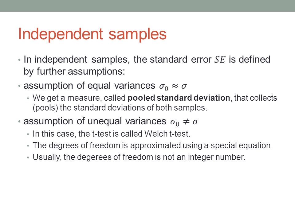
6 Independent samples

7

8 Výrobce garantuje, že jím vyrobené žárovky mají životnost v průměru 1000 hodin. Aby útvar kontroly zjistil, že tomuto konstatování odpovídá i v daném období vyrobená a expedovaná část produkce, vybral z připravené dodávky náhodně 50 žárovek a došel k závěru, že průměrná doba životnosti je 950 hodin se směrodatnou odchylkou 100 hodin. Je zjištěný rozdíl doby životnosti známkou nekvality produkce?

9 Ve Zpiťákově se dělal výzkum požívání alkoholu tak, že se náhodně vybralo 8 občanů a u nich se zjistila průměrná měsíční konzumace alkoholu. Po nějaké době došlo ve městě ke dvěma úmrtím na cirhózu jater (u jiných Zpiťarů, než kteří byli statisticky testováni). K posouzení, zda tato událost snížila konzumaci ve městě, se u stejných 8 občanů zjistila opět měsíční spotřeba. Rozhodněte, zda ona dvě úmrtí snížila konzumaci?

10 Průměrná váha žen v ČR ve věku 20-25 let je 67 kg se směrodatnou odchylkou 4 kg. Průměrná hmotnost 10 náhodně vybraných studentek VŠCHT činí 65,4 kg se směrodatnou odchylkou 3,2 kg. Vede dlouhotrvající sezení na nudných přednáškách a stres ze zkoušek z nesrozumitelných předmětů k poklesu váhy studentek?

11 Porovnáváme množství organických látek v odpadních vodách dvou papíren. Na základě několika náhodných měření v těchto papírnách máme rozhodnout, zda se tyto papírny liší v množství odpadních látek. V první papírně proběhlo 20 měření s průměrem 14,9 a směrodatnou odchylkou 4,8. 25 měření z druhé papírny vykazovalo průměr 22,0 a směrodatnou odchylku 7,4.

12 Podnikatel začal vyrábět jehly do šicích strojů. Prosadí se na trhu jedině tehdy, jestliže jeho jehly budou mít vyšší životnost než konkurenční. Z odborného tisku podnikatel zjistil, že životnost konkurenčních jehel je 8,72 milion stehů. Sám na zkoušku vyrobil 395 jehel, jejichž průměrná životnost činila 8,92 milionu stehů se směrodatnou odchylkou 1,81 milionu stehů. Má podnikatel rozjet výrobu naplno?

13 t-test in R t.test(x, y = NULL, alternative = c("two.sided", "less", "greater"), mu = 0, paired = FALSE, var.equal = FALSE, conf.level = 0.95 ) For the detailed description, see R manual at http://stat.ethz.ch/R-manual/R-patched/library/stats/html/t.test.html http://stat.ethz.ch/R-manual/R-patched/library/stats/html/t.test.html

14 One-sample t-test in R

15 x <- c(0.593, 0.142, 0.329, 0.691, 0.231, 0.793, 0.519, 0.392, 0.418) t.test(x, alternative="greater", mu=0.3) One Sample t-test data: x t = 2.2051, df = 8, p-value = 0.02927 alternative hypothesis: true mean is greater than 0.3 95 percent confidence interval: 0.3245133 Inf sample estimates: mean of x 0.4564444

16 Paired t-test A study was performed to test whether cars get better mileage on premium gas than on regular gas. Each of 10 cars was first filled with either regular or premium gas, decided by a coin toss, and the mileage for that tank was recorded. The mileage was recorded again for the same cars using the other kind of gasoline. Determine, whether cars get significantly better mileage with premium gas. reg <- c(16, 20, 21, 22, 23, 22, 27, 25, 27, 28) prem <- c(19, 22, 24, 24, 25, 25, 26, 26, 28, 32) t.test(prem,reg,alternative="greater", paired=TRUE) Paired t-test data: prem and reg t = 4.4721, df = 9, p-value = 0.000775 alternative hypothesis: true difference in means is greater than 0

17 Two-sample t-tests, independent samples

18 Assuming equal variances Control <- c(91, 87, 99, 77, 88, 91) Treat <- c(101, 110, 103, 93, 99, 104) t.test(Control, Treat, alternative=“less", var.equal=TRUE) Two Sample t-test data: Control and Treat t = -3.4456, df = 10, p-value = 0.003136 alternative hypothesis: true difference in means is less than 0

19 Assuming non-equal variances t.test(Control,Treat,alternative="less") Welch Two Sample t-test data: Control and Treat t = -3.4456, df = 9.48, p-value = 0.003391 alternative hypothesis: true difference in means is less than 0

20 Tests for the equality of the variances How we know if our variances are equal or not? We use the test of homogeneity of variances (also known as homoscedasticity). There exist several tests of homogeneity. I will start with F-test to introduce F-distribution (we will need this later in the lecture about analysis of variance). However, F-test is used very rarely as it strictly requires that the distributions are normal and it is not robust to the departures from the normality.

21 F-test of equality of variances source: Wikipedia

22 F-test in R x <- rnorm(50, mean = 0, sd = 2) y <- rnorm(30, mean = 1, sd = 1) var.test(x, y) F test to compare two variances data: x and y F = 2.5958, num df = 49, denom df = 29, p-value = 0.007395 alternative hypothesis: true ratio of variances is not equal to 1 95 percent confidence interval: 1.304183 4.883757 sample estimates: ratio of variances 2.595787

23 F-test is extremely sensitive to the departures from the normality. Alternative tests include Levene's test – performed over absolute values of the deviations from the mean, test statistic distribution: F-distribution Brown–Forsythe test – similar to Levene's test, but deviations from median are calculated, more robust The rationale for choosing amongst them is based on their performance at non-normal data. Levene's test is slightly more powerful than BF if the data really are normal, but not quite as robust if they aren't. Alternative tests of equality of variances

24 Power of the test A probability that it correctly rejects the null hypothesis (H 0 ) when it is false. Equivalently, it is the probability of correctly accepting the alternative hypothesis (H a ) when it is true - that is, the ability of a test to detect an effect, if the effect actually exists. Decision Reject H 0 Retain H 0 State of the world H 0 true Type I error H 0 false Type II error Probability of FN is β Probability of FP is α power = 1 - β

25 What factors affect the power? To increase the power of your test, you may do any of the following: 1. Increase the effect size (the difference between the null and alternative values) to be detected The reasoning is that any test will have trouble rejecting the null hypothesis if the null hypothesis is only 'slightly' wrong. If the effect size is large, then it is easier to detect and the null hypothesis will be soundly rejected. 2. Increase the sample size(s) – power analysis 3. Decrease the variability in the sample(s) 4. Increase the significance level (α) of the test The shortcoming of setting a higher α is that Type I errors will be more likely. This may not be desirable.