Statistické modelování v klinickém výzkumu Ladislav Pecen

Prezentace na téma: "Statistické modelování v klinickém výzkumu Ladislav Pecen"— Transkript prezentace:

1 Statistické modelování v klinickém výzkumu Ladislav Pecen

2 Klinický výzkum = výzkum aplikace nových léků v humánní medicíně.
Zjednodušeně Fáze I - farmakokinemitika* a farmakodynamika** na zdravých dobrovolnících Fáze II - účinnost léků u pacientů, pro které je určen Fáze III - vedlejší účinky léku, jeho tolerabilita Fáze IV - post-registrační vědecká či komerční fáze * Farmakokinetika = osud léčiva v organismu v časovém průběhu. - vstřebávání léčiva (absorpce) - jeho rozložení v těle (distribuce) - přeměna (metabolismus) - vzájemné ovlivňování (interakce) - vyloučení z organismu (eliminace - ledvinami, játry do žluči či stolice) ** Farmakodynamika = účinek léčiva na organismus

3 Některé milníky související s biostatistikou a klinickým výzkumem:
epidemie cholery v Londýně v roce mapování incidence -> identifikace závadného zdroje vody před 100 lety - založení journálu “Biometrics” (K.Person, F.Galton, W.F.R.Weldon) v roce1915 G.W.Snedecor organizoval první kurzy biometrie v roce 1951 A.B.Hill - první randomizovaný klinický (streoptomycin při léčbě tuberkulózy)

4

5 Cross-Sectional Studies
With outcome Subjects selected for the study (randomly from studied population) Without outcome Onset of study Time What is happening ?

6 Cohort Studies Exposed or subjects Cohort selected for the study
With outcome Without outcome Exposed or subjects Cohort selected for the study (randomly from studied population) With outcome Without outcome Unexposed or controls Onset of study Time What will happen?

7 Case - Control Studies Cases Controls Time Onset What happened ?
Exposed Unexposed Cases Exposed Unexposed Controls Onset of study Time What happened ?

8 Historical Cohort Studies
With outcome Without outcome Exposed or subjects Records selected for the study With outcome Without outcome Unexposed or controls Onset of study Time

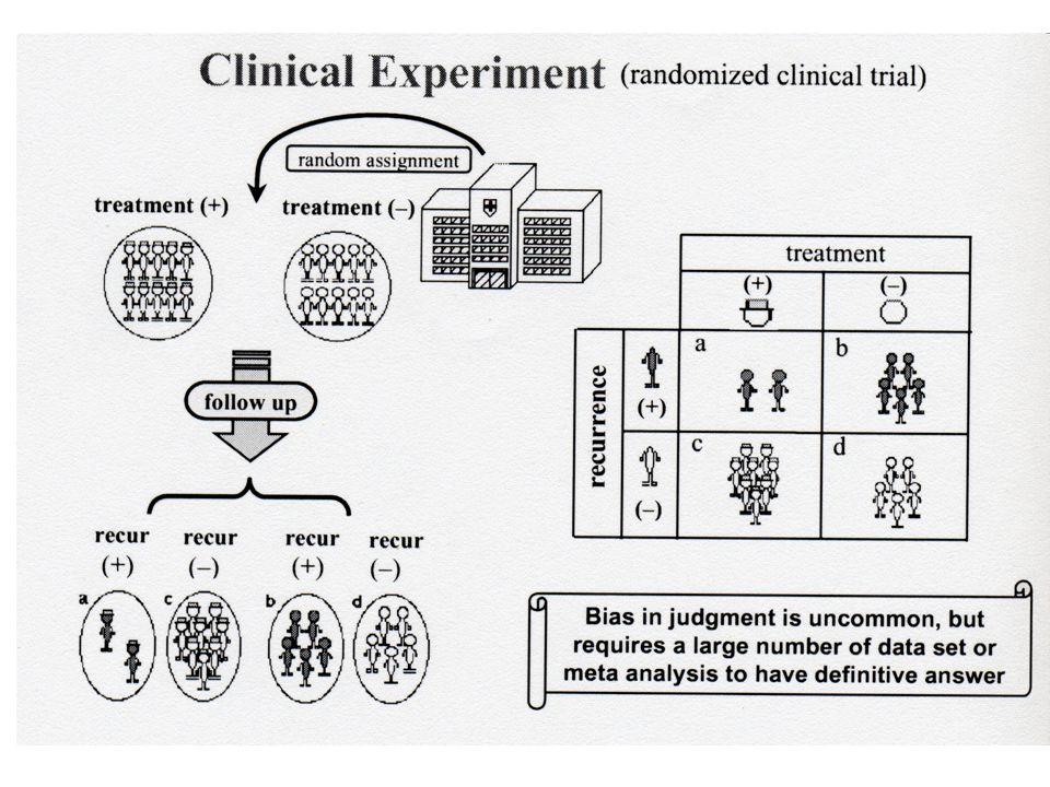
9 Randomized Clinical Trial Design
Experimental subjects With outcome Without outcome Subjects meeting entry criteria Randomization With outcome Without outcome Controls X X X X X X Onset of study Time Intervention

10 Clinical Trial with External Controls (including historical)
With outcome Without outcome Subjects With outcome Without outcome Results of Controls from previous (historical) study X X X X X X Onset of study Time Intervention in subjects only

11 Trial Design with Crossover
Experimental subjects Experimental subjects With outcome Without outcome With outcome Without outcome Subjects meeting entry criteria Randomization With outcome Without outcome With outcome Without outcome Controls Controls Washout period X X X X X X Time Onset of study Intervention Intervention

12 Self-controlled Trial Design (intervention -> placebo)
Subjects meeting entry criteria With outcome Without outcome With outcome Without outcome Washout period X X X X X X Time Onset of study Intervention Placebo

13 Self-controlled Trial Design (intervention->placebo->intervention)
With outcome Without outcome With outcome Without outcome Subjects meeting entry criteria With outcome Without outcome Washout period XXX XXX XXX Time Onset of study Intervention Placebo Intervention

14

15

16 Biostatistics in new treatment development
one-sided non-inferiority test is usually H0: difference in means < -d vs. H1: difference in means >= -d one-sided superiority test is usually H0: difference in means = vs. H1: difference in means >0, (to do power analysis it have to be in reality H1: difference in means >= d’). two-sided equivalence test H0: |difference in means | > d vs. H1: |difference in means | <= d two-sided non-equivalence test H0: |difference in means | <= d vs. H1: |difference in means | > d.

17 Studie Fáze I problémy bioequivalence
modely časového průběhu koncentrace účinné látky v krevní plazmě (v závislosti na dávce, jejím podávání, hmotnosti, pohlaví, věku apod.) - obvykle se jedná o parametrický model průběhu křivky a odhadují s jen parametry v rámci zvolené třídy průběhu křivek modely časových změn v závislosti na dávce a způsobu podání např. tepové frekvence a její variability u beta-blokátorů a antiaritmik EEG u neurofarmak (v používaných spektrálních pásmech) EKG predikční modely na odhad vzniku vedlejších efektů léčby (AEs)

18 Bioequivalence Drug plasma concentration Cmax AUC Tmax Time

19 Bioequivalence e.g. new treatment formulation - only test on healthy volunteers if time course of concentrations in blood is the same ->Y=ln(AUC) (Area Under the Curve of concentrations) instead of usual H0: E(YT - YR)= = 0 predefined equivalence region (-1,2) is used, typically 1=2, for FDA have to be used exp()=1.25. H0:   - or    <=> H01:   - and H02:    vs. HA = HA1  HA2 (HA1 is alternative to H01, HA2 to H02 ) => two one-sided hypotheses are simultaneously tested <=> 100-2 CI for  can be calculated - if completely inside (-, ) H0 - non-equivalence hypothesis is rejected. For =5% => 90% CI for  have to be used, p-value is the maximum of p-values of two one-sided hypotheses H01 and H02

20 Bioequivalence Standard approach - population bioequivalence - compare
just mean values of AUC (or logarithm of AUC) New approach H0:   - or    or T/ R   vs. H1: - <  <  and T/ R <  ; variation is also included Testing using maximal likelihood method (Vuorinen J., Turunen J: A simple three-step procedure for parametric and non-parametric assessment of bioequivalence. Drug Information Journal 31, pp , 1997). Individual equivalence H0 => more than means and variances different study design - 3 experiments per person, typically two times reference trt., one new trt., or randomly 2 R + 1 T vs. 1 R + 2 T, order is also random -> method of bootstrap is applied (Schall R., Luus H.G.: On population and individual bioequivalence. Statistics in Medicine 19, pp , 1993).

21 Fáze II problémy modelování účinnosti na pravostranně cenzorovaných datech (onkologie), či oboustranně cenzorovaných datech (AIDS/HIV) - zástupný (surrogate) indentifikátor progrese infekce - podmíněné funkce přežití (stochastické rizikové funkce) Response-surface modely pro kvantitativní (dávka) a kvalitativní proměnné a jejich kombinace nejtradičnější model je ANCOVA s baseline hodnotou jakou rušivým faktorem z důvodu nejnižšího relativního rozptylu (z třídy modelů ANCOVA, absolutní a relativní změna)

22 Synergism Analysis - the synergism definition: joint effect of two treatments being significantly greater than the sum of their effects when administered separately (positive synergism) or the opposite (negative synergism). Bootstrap technique: An aplication of resampling statistics. It is a data-based simulation method used to estimate variance and bias of an estimator and provide confidence intervals for parameters where it would be difficult to do so in the usual way. Evolutionary models - the estimation of time-dependence model of primary efficacy parameter during time based on dosages combination

23

24

25

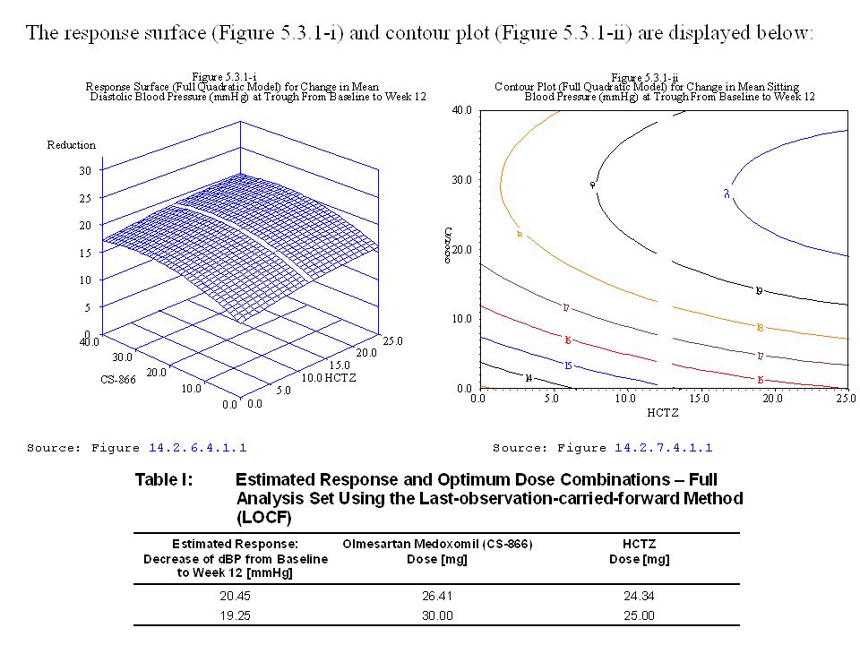
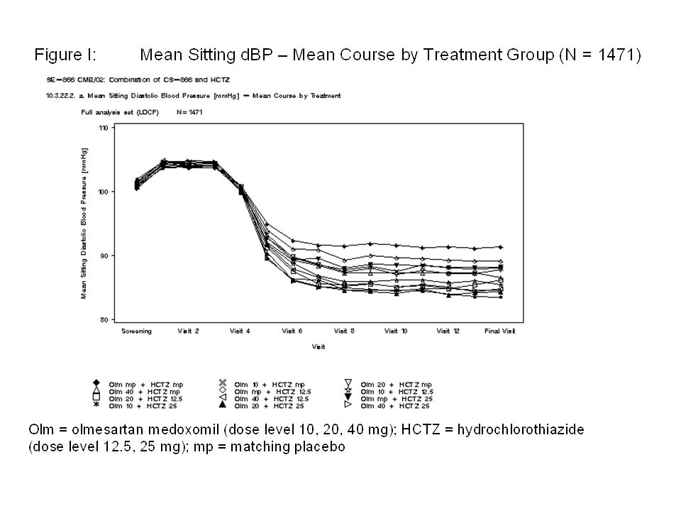
26 Parametric response surface model Example:
The mean change from baseline to week 12 in mean sitting dBP at trough analysed using response-surface methodology. This approach aims to predict an optimum dose combination within the continuous response surface. The relationship between CS-866 and HCTZ and the dose combinations will be examined using the quadratic model: Y = 0 + 1X1 + 2X2 + 3X12 + 4X22+ 5X1X2 where Y=mean change from baseline to week 12 in mean sitting dBP at trough; X1=dose of CS-866 and X2=dose of HCTZ. Quadratic and interaction terms that are not statistically significant will be removed from the model in a stepwise fashion until only statistically significant terms remain (p-value  0.05). Response-Surface Model is just special case of polynomial (generally non-linear, in our case polynomial in 2nd power) multidimensional regression model. Adjustment allowing to exclude influence of confounding factor could be used. Non-parametric response surface model Smoothing procedure

27 Oncological Trials-Assessing risk of an event
In oncology the target variable of interest (primary efficacy variable) is usually survival time, disease-free, metastases-free time or a similar time-to-an-event => survival analysis models. Assessing the risk of progression, the risk of occurrence of metastases etc for a given patient and time instant. We are able to quantify the risk of the patient but 95% CI for probability of an event for the patient is 0% - 100%. Techniques: Kaplan-Meier estimation of survival function, Cox proportional risk model or Aalen additive risk model,accelerated life model, competing risk model.

28 HIV/AIDS related studies
The target variable of interest is survival time - the data are left-time censored (time of infection or sero-conversion is unknown) or left-time interval censored (date of last negative and first positive tests are known), right-time censored (death date is sometimes unknown) => survival analysis models with both sides censored data. Using of surrogate indicator of infection progression - e.g., CD4+ T-lymphocytes, No of virus RNA copies Complicated model for many simultaneous treatment effect modeling. New AIDS treatment - Fuzeon produced by Roche Holding (price about USD = Euro per year, fuse inhibitor)

29 Ordinal categorial data
e.g back pain intensity assessed by five-point verbal rating scale (VRS-5) (0= mild, 1= discomforting, 2= distressing, 3= horrible, 4= excrutiating); functional capacity score after performing activity - e.g., putting on a jack, assessed using a four-point scale (1= without pain, 2= with slight pain possible, 3= interrupted pain, 4= impossible because of pain) - 2 test ignore the ordinality of categories - rank tests (e.g. Wilcoxon Rank-Sum test) - small No of categories - ordinal regression models - Proportional Odds ratio (POR) - generalization of binary logistic regression - works with cumulative probabilities - Continuation Ratio (CR) - works with conditional probabilities (hazards) Details Armstrong B., Sloan M.: Ordinal regression models for epidemiologic data, Amer.Jour.of Epidem. 129, pp ,1989

30 Statistical models based on family tree structure - e.g.,
for colorectal cancer cases (black below) example of one family tree: For statistical analyses one need: 1. Families-tree with hereditary incidence (typically 2 and more cases as a average number at any sub-tree parents + children 2. Control group - families without occurrence of the particular disease 3. Families with probably random disease occurrence (just one case of the particular disease, or occurrence and not in group 1.)

31 Used symbols definition:

32 More difficult family structure

33 Typical results based LOD score statistical technique:
Particular Disease Related Genes (Genes mutations) Particular Disease Protective Genes (Genes mutations)

34 BRCA-I and BRCA-II gene mutations and breast cancer incidence